INDEX

• introducation to Excel
• Features of Excel
• Features in Excel
• Data visualization
• Pivot Tables in Excel
• Data Analytics Tool in Excel
• Excel Macros
• Shortcut & Tips in Excel

INTRODUCTION TO EXCEL

• Microsoft Excel is a powerful spreadsheet software developed by miscrosoft, part of the microsoft office suite ( now also available as part of the Microsoft 365).
• it is used for organizing , analyzing, and visualizing data in tabular form.
• Excel allows users to creat spreadsheets with multiple worksheets, perform complex calculations, generate charts and graphs, and automate takes through macros and formulas.

FEATURTES OF EXCEL

1.workbooks and worksheets:

• Excel organizes data in workbooks, which contain multiples worksheets.
• Each worksheets is made up of rows and columns forming a vgrid where data is entered.

2. Formulass and functions:

• Excel supports a wide range of formulas and functions to perform calculations on data

3.Data Analysis tools:

• Excel provides tools such as pivot tables, conditional formatting, and data validation to analyze and interpret data effectively.

4.charts and graphs:

• Excel can generate various types of chats ( e.g., bar, line, pie charts ) to visually represent data and trends, makling it easier to understand and present.

5.Automation and macros:

• With VBA (visual basic for applications), Excel allows users to automate repetitive tasks by creatingmacros-scripts that run a series of commands automatically.

FUNCTIONS IN EXCEL

in excel, functions are predefined formulas that allow you to perform various calculations and operations easily.

1.MATHEMATICAL FUNCTIONS

sum: Adds up a range of cells. ( Ex: =sum[A1:A5] )

AVERAGE: Calculates the average of a range of cells. Ex: =AVERAGE (A5:A10)

COUNT: Counts the number of cells containing numbers. Ex: =COUNT(A10:A14)

MIN: Finds the smallest value in a range. Ex: = MIN(A15:A18)

MAX: Finds the largest value in a range. Ex: =MAX(A20:A30)

MOD: Returns the remainder after division. Ex: =MOD(A14:A19)

ROUND: Rounds a number to a specified number of decimal places.

Ex: =ROUND(A1:A10)

2. TEXT FUNCTIONS

CONCATENATE: Combines multiple text strings into one. Ex: =CONCATENATE (A1, ” “, B1)

LEFT: Extracts a specified number of characters from the left of a text string. Ex:- =LEFT(A1, 5)

RIGHT: Extracts a specified number of characters from the right of a text string. Ex: – =RIGHT(A1, 3)

UPPER: Converts text to uppercase. Ex: – =UPPER(A1)

LOWER: Converts text to lowercase. Ex: – =UPPER(A1)

FIND: locate text within a string. EX:FIND(","ANJIRAJU")//returns 5

REPLACE: Replace existing text using a position EX:=REPLACE("XYZ123"4,3,"ABC")//returns"XYZABC"

TRIM: Remove extra spaces from text. EX;=TRIM(" ANJIRAJU.")//returns"ANJIRAJU."

LEN: count the number of characters in a string. EX;=LEN("ANJIRAJU")//returns 8

3.LOGICAL FUNCATIONS

IF: Performs a conditional test and returns one value if true
and another if false.

EX : = IF (A1>10,"Yes","No")

AND : Returns TRUE if all conditions are true.
Ex: – =AND(A1>5, B1&It;10)

OR: Returns TRUE if at least one condition is true.
Ex: – =OR(A1>5, B1<10)

NOT: Reverses the logic of its argument (TRUE becomes
FALSE, and FALSE becomes TRUE).
Ex: -NOT(A1>10)

SWITCH: – The Excel SWITCH function compares one value
against a list of values and returns a result corresponding
to the first match found. When no match is found, SWITCH
can return an optional default value.

EX: – = SWITCH

(TURE,A1>=100,qout;Gold",A1>=500"sliver"sliver"Bronze&quote

4. DATE & TIME FUNCTIONS

TODAY: Returns the current date. Only date is display.
Ex: – =TODAY()

NOW: Returns the current date and time.
Ex: – NOW()

DATE: Returns the date based on year, month, and day inputs.
Ex: – =DATE(2024, 12, 20)

YEAR: Extracts the year from a date.
Ex: – = YEAR ("23-aug-2012")//returns 8

MONTH: Extracts the month from a date.
Ex: – = MONTH ("23-Aug-2012") // returns 8

DAY: Extracts the day from a date.
Ex: – = DAY (2022-11-25) // returns 11

DATEDIF: – Get days, months, or years between two dates
Ex: – =DATEDIF: – Get days, months, or years between two dates

EX:-=DATEDIF("1-Jan2022"1-Mar2024","1-Mar2024","y")//returns 2 years =DATEDIF("1-Jan-2022","1-Mar2024","m")//retuns 26 months=DATEDIF("1-Jan-2022&qout;,"1-Mar2024"d")//returns 790 Days

5. LOOKUP & REFERENCE FUNCTIONS

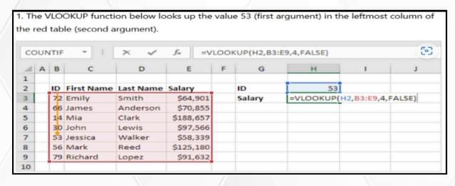
VLOOKUP:- Searches for a value in the first column of a
table and returns a value from another column in the
same row.
EX:

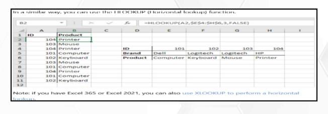
HLOOKUP: – Like VLOOKUP but searches horizontally in the
first row.

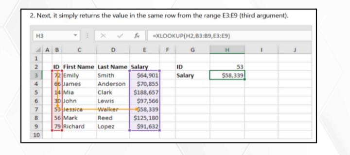
XLOOKUP: – XLOOKUP is a modern replacement for the
VLOOKUP function. It is a flexible and versatile function that
can be used in a wide variety of situations. XLOOKUP can
find values in vertical or horizontal ranges, can
perform approximate and exact matches, and supports
wildcards (* ?) for partial matches

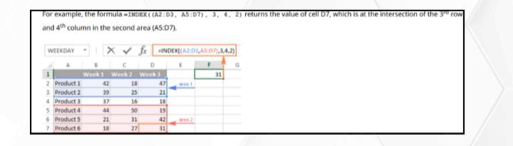
INDEX: Returns the value of a cell in a specific row and
column ofa range

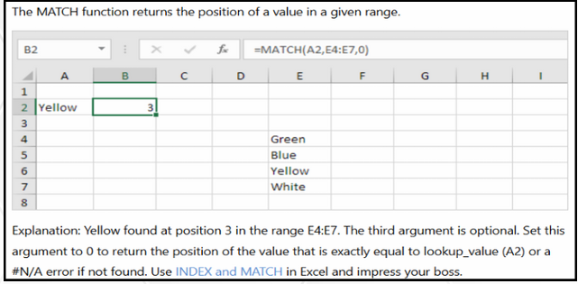
MATCH: Searches for a value in a range and returns its
relativeposition.

DATA MANIPULATION IN EXCEL

Data manipulation in Excel involves various techniques
to organize, analyze, and transform data to make it
more usable and insightful.
It can include sorting, filtering, formatting, combining
data, and using formulas to transform and summarize
data.

1. SORTING DATA
   Ascending or Descending Order: Sorting data helps
   organize it in a meaningful order, either alphabetically or
   numerically.
   How to Sort:
   Select the range of data.
   Go to the Data tab.
   Use the Sort A to Z (ascending) or Sort Z to A
   (descending)buttons.
   Custom Sorting: If you want a custom order (e.g., days of
   the week), you can set custom sorting

2. FILTERING DATA

AutoFilter: Filters data to display only the rows that meet
certain criteria.

How to Filter: Select your data range (including headers).
Go to the Data tab and click on Filter.
Use the dropdowns in each column header to set your
filter conditions.

You can filter by: Text (e.g., contains, starts with)
Numbers (e.g., greater than, less than)
Dates (e.g., before, after a specific date)

Advanced Filter: More complex filtering, where you can
use multiple criteria and even extract data to another
location.

How to Use: Go to Data > Advanced (in the Sort & Filter
group) and configure the filter criteria

3. USING CONDITIONAL FORMATTING

Highlighting Data: You can automatically apply different
formatting to data based on certain conditions.

How to Apply:
Select your data range.
Go to Home tab > Conditional Formatting.
Choose from options like Highlight Cell Rules, Data Bars,
Colour Scales, etc.

Example: Highlight cells that are greater than a certain value or have duplicate values.

4. DATA VALIDATION

Setting Data Validation: Ensure that only valid data is entered into cells (e.g., only numbers, dates, or specific
choices).

How to Set: Select the range.
Go to Data tab > Data Validation.
Define the type of data allowed (e.g., whole
numbers,dates, or a custom rule).

Drop-Down Lists: Allow users to select from predefined
values.

Example: Go to Data Validation, select List, and provide a
range ormanually input the options

5. PIVOT TABLES FOR DATA SUMMARY

Create Pivot Tables: Pivot Tables are a powerful way to summarize and manipulate large sets of data. You can group, filter, and aggregate data dynamically.

How to Create a Pivot Table:
Select your data range. Go to Insert tab > PivotTable. Drag and drop fields into rows, columns, values, and
filters to organize and summarize your data.

Example: Summarize sales by region and product

6. TEXT-TO-COLUMNS

Split Data: Split data in a column into multiple columns, such as splitting a full name into first and last names.

How to Set: Select the column. Go to Data tab > Text to Columns. Choose either Delimited (if there is a specific separator likecommas or spaces) or Fixed width (split based on specificpositions).

7. REMOVING DUPLICATES

Remove Duplicates: Clean up your data by removing duplicate entries.

How to Remove: Select your data range. Go to Data tab > Remove Duplicates. Choose which columns to check for duplicates.

8. CONSOLIDATING DATA

Consolidate Data from Multiple Sheets: Combine data from multiple ranges or sheets into one summary table.

How to Consolidate:Go to Data tab > Consolidate. Choose the function (e.g., sum, average) and the
ranges to
consolidate.
Using Formulas: You can also consolidate data manually using formulas like SUMIF, VLOOKUP, INDEX, etc.

9. GROUPING AND UNGROUPING DATA

Group Data: You can group rows or columns to collapse or expand data for better organization.

How to Group:
Select the rows or columns.
Go to Data tab > Group.

Ungroup Data: To expand the grouped data, select the
grouped rows/columns, and click Ungroup.

10. CONVERTING DATA TYPES

Convert Text to Numbers: Sometimes numbers stored as text need to be converted to actual numbers for
calculations.

PART 2 UPCOMING TOPICS

• DATA VISUALIZATION
• PIVOT TABLES IN EXCEL
• EXCEL MACROS
• SHORTCUTS AND TIPS IN EXCEL